Identification with DAGs: Introduction with simple simulations
Untitled
In this post I want to share with you some introductory ideas on how Directed Acyclical Graphs (DAGs) are used for causal identification. I am also sharing a few (Stata based) numerical simulations (here), that can be illustrative of their use in a regression application.
The DAG approach has been around for more than fifteen years now, and is described in extent in the excellent book by Pearl and Mackenzie (2018)’s “The Book of Why”. There’s so much going on in the book that I will be writing more about it in a future post.
For those that are completely unfamiliar with the framework, DAGs are used to represent assumptions on the causal relationship between theoretical constructs (and their variables), and then, using the resulting graphs, to identify causal identification strategies. In observational settings, where we are used to think about possible confounders which introduce bias in the measured effects of interest, Pearl’s approach proposes a method on how and when to de-confound.
Let me give a few examples on how these graphs work, and what the simulations I am attaching show.
Let’s assume that we are in an observational setting and are interested in the identification of the effect of variable X on variable Y. Let’s also assume that there is also a variable Z which has an effect on X and Y. This is the basic story on the well known confounder bias idea, and is represented in the following graph:
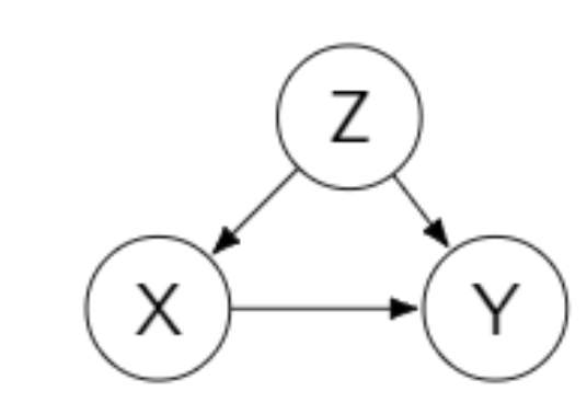
In order to identify the effect of X on Y we need to control for Z. Controlling for Z, which consists in examining the relationship between X and Y, having fixed the value of Z, blocks the confounder effect of Z. (1). Confounding occurs because there is an alternative path that connects X and Y. Pearl uses the analogy of a pipe: the idea is that incorporating Z as a control blocks the alternative pipe X<=Z=>Y. In referring to this alternative path he also refers to it as a “back-door path”.
In a regression framework adding controls is equivalent to adding the variable as an explanatory regressor. For the following simulated scenario, let’s assume that there is no causal relationship between X and Y, and that both variables are (linearly) influenced by by the confounder. For instance, assume that
Where , and are random uniform noise.
Now assume that, in trying to identify the effect of X on Y we estimate the model where we ommit Z. The result is:

The coefficient for X suggests that there is a negative effect. This is actually not surprising giving our model: if Z has a negative effect on X and a positive effect on Y, in the absence of Z a negative relationship between X and Y is observed.
Now lets add the control for Z, and estimate:
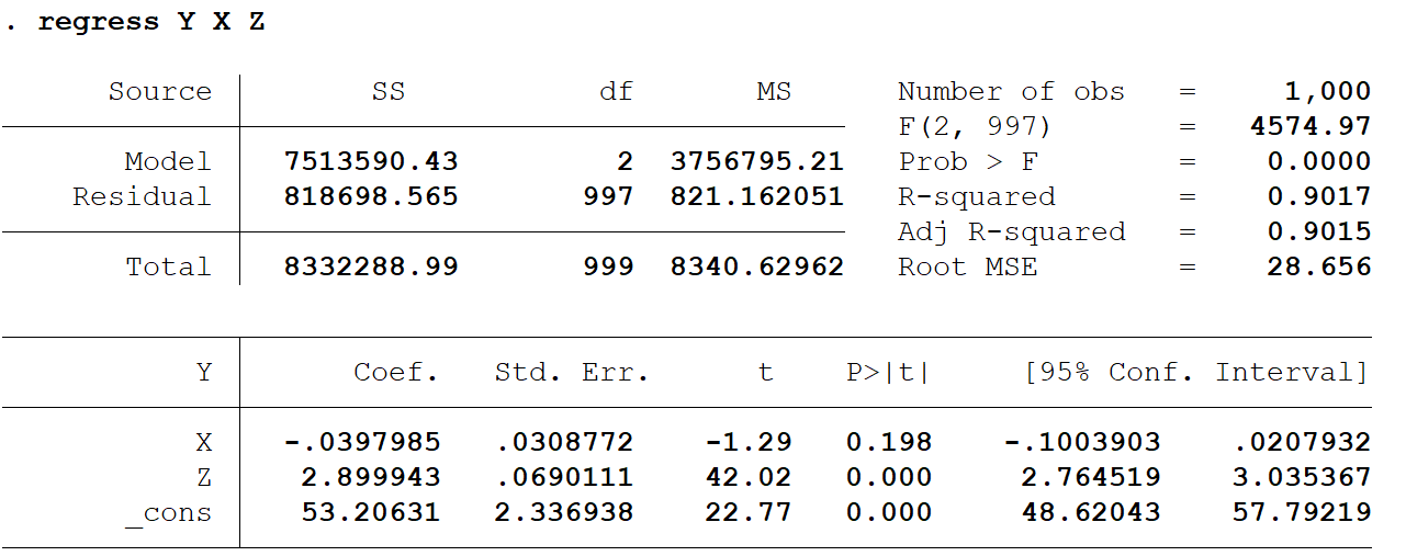
We can see that the spurious effect disappears: the coefficient for X is now close to 0, and the coefficient for X is close to 3.
Bad control: introducing a collider
Consider now the following example, which is a slightly modified version of one of the cases introduced in the book.
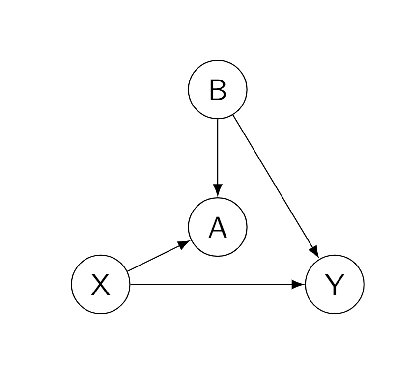
In this situation, a possible pipe connects X and Y. This is the pipe X=>A<=Z=>Y. But there is something special about this pipe. Whenever there is a node when two causal connections collide (such as in: =>A<=), there is no possible flow of information. This is what Pearl calls a collider. Then, if that were the unique relevant pipe in the flow, there would be no need of adding controls, because the pipe is already blocked.
The problem appears if you control for A. The effect of controlling with a collider is the opposite: controlling for A will open the pipe and allow the flow of information through the confounding pipe.
Now lets implement this situation in a simple simulation. Lets assume
Where and is random noise.
Let’s first note that we do not need to introduce controls when identifying the effect of X on Y.
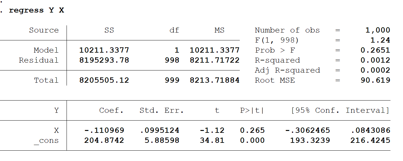
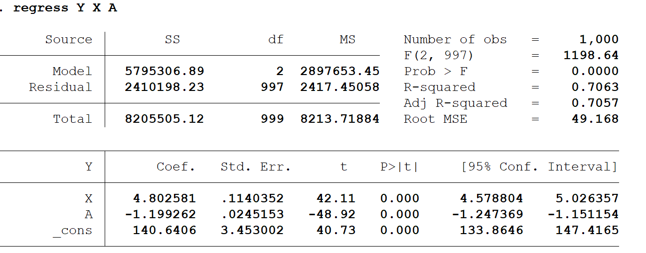
Now, if A is added as control, the back-door path is opened, and a bias emerges!
We can close the back-door path again, by also controlling for B.

In the github repository you will find some more examples. I will be adding more real examples in the future, as well as more comments in the book, so stay tuned! If you are interested in these methodologies don’t go without leaving your comments.
- More precisely, the relationship between X and Y would be evaluated at each level of Z, and the an average weighting the relative importance of each value of Z would be performed
En este post, quiero compartir con ustedes algunas ideas introductorias sobre cómo se utilizan los Gráficos Acíclicos Dirigidos (DAG) para la identificación causal. También estoy compartiendo algunas simulaciones numéricas (basadas en Stata) aquí, que pueden ser ilustrativas de su uso en un contexto de identificación causal usando regresión.
El enfoque de DAG se describe en gran medida en el excelente libro de “The book of Why” de Pearl y Mackenzie (2018). A mi entender el libro es tan rico en ideas que seguramente escriba más sobre el mismo en el futuro.
Para aquellos que no están familiarizados con el marco, los DAG se utilizan para representar suposiciones sobre la relación causal entre constructos teóricos (y sus variables), y luego, utilizando los gráficos resultantes, para identificar estrategias de identificación causal. En casos de trabajo con datos observacionales, donde estamos acostumbrados a pensar en posibles factores de confusión que introducen sesgos en los efectos de interés medidos, el enfoque de Pearl propone un método sobre cómo y cuándo se debe confundir.
Permítanme dar algunos ejemplos sobre cómo funcionan estos gráficos y qué muestran las simulaciones que adjunto.
Supongamos que estamos en un entorno de observación y nos interesa la identificación del efecto de la variable X en la variable Y. También supongamos que también hay una variable Z que tiene un efecto en X e Y. Esta es la historia básica de la conocida idea de sesgo de confusión, y se representa en el siguiente gráfico:
Para identificar el efecto de X en Y, debemos controlar Z. El control de Z, que consiste en examinar la relación entre X e Y, habiendo fijado el valor de Z, bloquea el efecto de confusión de Z. (1). La confusión se produce porque hay una ruta alternativa que conecta X e Y. Pearl utiliza la analogía de una tubería: la idea es que la incorporación de Z como control bloquee la tubería alternativa X <= Z => Y. Al referirse a este camino alternativo, también se refiere a él como un “camino de puerta trasera” (back-door path).
En un marco de regresión, agregar controles es equivalente a agregar la variable como un regresor explicativo. Para el siguiente escenario simulado, supongamos que no hay una relación causal entre X e Y, y que ambas variables están influenciadas (linealmente) por el confusor. Por ejemplo, supongamos que
Donde , and son ruido uniforme.
Ahora asuma que, en intentar identificar el efecto de X sobre Y se estima el modelo: donde omitimos Z. El resultado es:
El coeficiente para X sugiere que hay un efecto negativo. En realidad, esto no es sorprendente con nuestro modelo: si Z tiene un efecto negativo en X y un efecto positivo en Y, en ausencia de Z se observa una relación negativa entre X e Y.
Ahora añadimos Z, y estimamos:
Podemos ver que el efecto espurio desaparece: el coeficiente para X ahora está cerca de 0, y el coeficiente para X está cerca de 3.
Mal control: introduciendo un colisionador
Considere ahora el siguiente ejemplo, que es una versión ligeramente modificada de uno de los casos presentados en el libro.
En esta situación, un posible conducto conecta X e Y. Este es el conducto X => A <= Z => Y. Pero hay algo especial en esta tubería. Siempre que hay un nodo cuando dos conexiones causales chocan (como en: => A <=), no hay un posible flujo de información. Esto es lo que Pearl llama un colisionador. Entonces, si ese fuera el único tubo relevante en el flujo, no habría necesidad de agregar controles, porque el tubo ya está bloqueado.
El problema aparece si controlas por A. El efecto de controlar con un colisionador es el opuesto: el control de A abrirá la tubería y permitirá el flujo de información a través de la tubería de confusión.
Ahora vamos a implementar esta situación en una simulación simple. Asumamos
Donde y es ruido aleatorio.
Primero notemos que no necesitamos introducir controles al identificar el efecto de X en Y.
Ahora, si se agrega A como control, se abre el camino de la puerta trasera y surge un sesgo!
Podemos cerrar el camino de la puerta trasera nuevamente, controlando también por B.
En el repositorio de github encontrarás más ejemplos. Estaré agregando más ejemplos reales en el futuro, así como más comentarios en el libro, ¡así que estad atentos! Si estás interesado en estas metodologías no te quedes sin dejar tus comentarios.
- More precisely, the relationship between X and Y would be evaluated at each level of Z, and the an average weighting the relative importance of each value of Z would be performed